Talk:Search Odds/chi square tutorial for excel
This is a (hopefully) easy to understand walkthrough on how to perform the two types of chi square analyses, using a simple spreadsheet program. To show people, we'll be using two easy, simple data sets:
- the Drug Store (Bargain Hunting) data set, for single-set analysis
- the Cathedral and Church data sets for multi-set analyses.
Explanations
Now, before we get started, we'll try to explain a few things about the test that we are using.
Why chi square?
Why use a chi square analysis over some of the other types of tests? There are several good reasons. Chi square analyses are considered the best analysis for data with the following features:
- The data is collected in categories that cannot be "counted" per se, but are more correctly labels.
- The data is discrete (ie, only certain values are allowed for it, and one cannot make a score between these values)
- The distribution of the data is not a normal distribution (ie a bell curve)
The data we are looking at fits all three of these features. Our categories are (depending on your view) either the search result or the location searched. We cannot find "half a gun", we are restricted to whole numbers, thus we are working with discrete data. Further, we cannot claim that our data is a normal distribution between categories.
How does a chi square analysis work?
A Chi-square test is in many ways a restricted test - it does not use mean or variance (the major components of most major statistical analyses), for the main reason that it makes no assumptions about the underlying data. Instead, it tests how well the data fits a hypothesised data set. It does this by picking up differences between the observed data in each category, and the hypothesised data set, and then adds each of these differences together, to form a general difference score.
We can then use this score to figure out the probability that the deviation from the data set could have happenned by chance. If the difference number is not above a specified number we're looking for, we must assume that the deviations are by chance, and thus the data fits the distribution we were testing. We'll discuss exactly how we do that later on.
Single-set Analysis
We'll start with the simplest form of analysis - comparing a single set of data to our hypothesised analysis. To do this, we'll pick our simplest data set - Drug Store (bargain hunting). Before we start, you'll need to take this data set, and paste it into Excel.
Step 1: Hypothesis
Before we begin any calculations, we should decide on what, exactly, we're looking for, and state it as a hypothesis. Since most analyses are built towards finding differences, we need to build our hypothesis as us looking for differences between our data set and the hypothesised distribution. So, our Hypothesis is:
- H(1): That the data deviates significantly from the hypothesised distribution of 35% First Aid Kits, and 65% Failed searches.
This allows us to find a Null Hypothesis, as follows:
- H(0): That the data does not deviate significantly from the hypothesised distribution of 35% First Aid Kits, and 65% Failed searches.
We now have two possible hypotheses that we'll be testing. At the end of the test, we will choose one of them to be our conclusion of the test.
Step 2: Summarising the Observed Data
At this point, you should have the data we're working on pasted into excel. If you haven't done so already, use SUM() to grab the three totals. You should also record the distribution we're looking for (in this case, .35 for First Aid Kits, and .65 for Failed searches). At start, you should have a work field (where most of our calculations are going to take place) as follows:
Next, put your sums in each category. It should now look like this:
Step 2: Making the Expected Data
Next, we need to create data that fits our test distribution. The best way to do this is to take the number of searches (your grand total), and in each category, multiply it by the fraction we want to test. (so, multiply the total by .35 in the First Aid Kit category, and by .65 in the Failure category. To do this in Excel, we just do =[location of total]*[location of fraction]. So, like the following:
Make sure you do this to the other field, and (very importantly), use SUM() to add up all the expected data, and make sure it equals the same as our observed data's sum. Once this is done, our workspace should look like this:
Step 3: Calculating the Difference
And now, we can begin getting into the real analysis. For each category, we need to find the square of the difference between our two values, divided by the expected value. The resultant value is the magic bit of this test - it simultaneously picks up the differences in our test data, and then, by dividing it against our expected value, it standardises the data into a specific probability curve. So, regardless of the size of each category, we can make clear comparisons regarding the differences from their best fit.
As a note, we're almost certain that the data will not perfectly fit, simply due to sampling error. So we're more correctly trying to determine if the lack of fit is high enough to suggest that the sample is from a different population to the one we think it's from.
The equation you'll need for each category will take the form
- =(([observed]-[expected])^2)/[expected]
So, with our workspace, the equation looks like:
We now do this for every category we have, and then sum each result that we get. So, the workspace should look like:
And now, we have our chi-square value! That sum you did of each result has now become our chi-square value. In this case, it's 0.442248
Step 4: Finding out it's significance
The final step is determining whether the value we have indicates a significant deviation from our expected values. We need one more piece of data before we can do this: The Degrees of Freedom of the data.
Degrees of Freedom: A quick explanation
Degrees of Freedom sounds like a scary concept, but in fact it's quite straighforward. We have a collection of data, and one important piece of information: the sum of that data. Now, there are a lot of sets of data that could equal up to that sum, so we could say that the data is free to move quite a bit, and that the two values could be anything we want and still have that sum.
In fact that's not quite right - only one of those values is free to move. Because once we've figured out one value, in order for the sum to still be correct, the other value must be a number that, when added to the first value, totals our sum.
We can actually show that this is true for any number of values. If we have 5 numbers that total a specific number, we can let the first four values be anything we want - but the 5th number must be a number which, when added to the first four values, total our sum.
So, our Degrees of Freedom, therefore, must be one less than the number of categories we're testing. Simple as that. So, in our case, our Degrees of Freedom equals 1.
Probability test
Now that we have our chi square value and our Degrees of Freedom, we can now find the probability value of the data we have. Normally, one would look up in a big chi square table, but fortunately for us, there is a calculator on the web that will do the hard work for us:
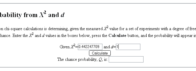
We thus copy our chi square value and our degrees of freedom into the calculator as follows:
Then press the button to get the result. In this case, it's 0.5060. So, there's about a 1 in 2 chance of the observed data emerging from the distribution we're testing by chance. Not bad odds. In general, hypothesis testing requires that the number be smaller than an arbitrary probability of chance in order for it to be clear that there are differences. In social sciences, 0.05 is the probability that's normally chosen, ie less than a 1 in 20 chance of occuring by chance. This is a reasonable milestone for our work, so we'll compare our result to this. Of course, looking at our probability result, we're not even close. It's pretty clear that the data we observed is fairly close to what we expected. Thus, we do not reject our H(0) - it was right all along!
Multiple-set Analysis
In this form of the chi square, we're doing something a little different. Instead of comparing an observed set to a set distribution, we're actually comparing two sets of observational data. For this exercise, we're going to attempt to find out whether there is a difference between Lights on and Lights off data in Necrotech Buildings.
Step 1: Hypothesis
Before we begin any calculations, we should decide on what, exactly, we're looking for, and state it as a hypothesis. Since most analyses are built towards finding differences, we need to build our hypothesis as us looking for differences between our data set and the hypothesised distribution. So, our Hypothesis is:
- H(1): That there is a significant difference between Lights on and Lights off data.
This allows us to find a Null Hypothesis, as follows:
- H(0): That there is not a significant difference between Lights on and Lights off data.
We now have two possible hypotheses that we'll be testing. At the end of the test, we will choose one of them to be our conclusion of the test.
Step 2: Summarising the Observed Data
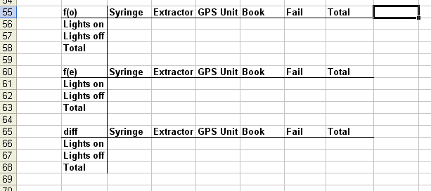
At this point, you should have the data we're working on pasted into excel. We want to collect each criteria into separate totals this time, so our field is going to be a little larger, like so:
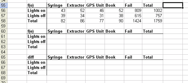
Next, put your sums in each category for dividing between the two groups, I'll note that SUMIF() is a very useful function, and you should use Excel's help to get familiar with it. Once you're done, your workspace should look like this.:
Step 2: Making the Expected Data
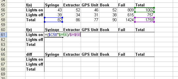
Next we need to make our expected data - the data that we would expect would emerge, if there was no difference between the two distributions. This seems daunting, but happily, there's a very simple formula that will allow you to calculate what this value is for every cell:
- E = ((row total)*(column total))/(grand total)
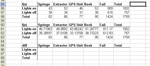
As such, you'll need to use your observed data space to do this. So, something like the following:
Make sure you do this to every cell, and (very importantly), use SUM() to add up all the expected data, and make sure it equals the same as our observed data's sum. Once this is done, our workspace should look like this:
Step 3: Calculating the Difference
And now, we can begin getting into the real analysis. For each cell, we need to find the square of the difference between our two values, divided by the expected value. The resultant value is the magic bit of this test - it simultaneously picks up the differences in our test data, and then, by dividing it against our expected value, it standardises the data into a specific probability curve. So, regardless of the size of each category, we can make clear comparisons regarding the differences from their best fit.
As a note, we're almost certain that the data will not perfectly fit, simply due to sampling error. So we're more correctly trying to determine if the lack of fit is high enough to suggest that the sample is from a different population to the one we think it's from.
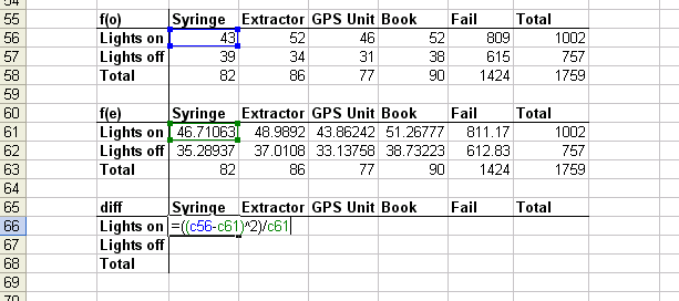
The equation you'll need for each cell will take the form
- =(([observed]-[expected])^2)/[expected]
So, with our workspace, the equation looks like:
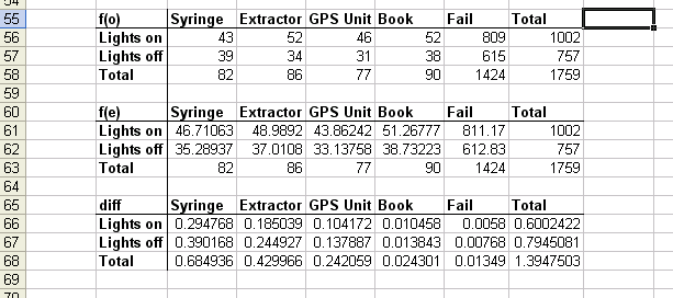
We now do this for every cell we have, and then sum each result that we get. So, the workspace should look like:
And now, we have our chi-square value! That sum you did of each result has now become our chi-square value. In this case, it's 1.3947503
Step 4: Finding out it's significance
The final step is determining whether the value we have indicates a significant deviation from our expected values. We need one more piece of data before we can do this: The Degrees of Freedom of the data. In this case, all you need to remember is that df = (no. of columns - 1)*(no. of rows - 1). So, in our case, our df = 4.
Probability test
Now that we have our chi square value and our Degrees of Freedom, we can now find the probability value of the data we have. Going through the previous website, we can look up the same thing, and it turns out our probability is 0.8451. Fairly clearly, there's no significant difference between the two groups. Thus, we do not reject our H(0) - it was right all along!
Questions
[If people are still confused, post here and I'll try to explain better. -- Odd Starter talk | Mod | W! ]


